vistan.algorithm(
    vi_family = "rnvp",
    full_step_search = True,
    full_step_search_scaling = True,
    step_size_exp = 0,
    step_size_exp_range = [0, 1, 2, 3, 4],
    step_size_base = 0.1,
    step_size_scale = 4.0,
    max_iters = 1000,
    optimizer = 'adam',
    M_iw_train = 1,
    M_iw_sample = 10,
    grad_estimator = "STL",
    per_iter_sample_budget = 100,
    fix_sample_budget = True,
    evaluation_fn = "IWELBO",
    rnvp_num_transformations =  10,
    rnvp_num_hidden_units =  32,
    rnvp_num_hidden_layers =  2,
    rnvp_params_init_scale =  0.01
)Note: Since writing this post, Pathfinder (described below as well in Section 5) has become available in CmdStan, which poses a problem for this concluding post to the series.
More specifically, the running example (a simple-ish MRP model), was chosen to be too complex to get a good approximation with a simple mean-field or full-rank approximation as implemented by rstanarm, but Pathfinder is both significantly faster than what’s below, and quite capable here.
This is a bit awkward, but is informative. I generally still endorse my thoughts below about how to make variational inference work for much more complex models. That said, the series example now lives in an awkward middle ground where the most basic methods fail, but middle of the road options like Pathfinder can outperform complex methods like those I spent the series introducing.
Another point worth emphasizing here is that the methods below are not only inefficient compared to Pathfinder, they produce worse posteriors with regards to uncertainty! This highlights that more complex tools for variational inference are not uniformly better for all problems, even if something like the methods below might still be in my toolbox for more challenging models.
This is the final post in my series about using Variational Inference to speed up complex Bayesian models, such as Multilevel Regression and Poststratification. Ideally, we want to do this without the approximation being of hilariously poor quality.
The last few posts in the series have explored several different major advances in black box variational inference. This post puts a bunch of these tools together to build a pretty decent approximation that runs ~8x faster than MCMC, and points to some other advances in BBVI I haven’t had time to cover in the series.
The other posts in the series are:
- Introducing the Problem- Why is VI useful, why VI can produce spherical cows
- How far does iteration on classic VI algorithms like mean-field and full-rank get us?
- Problem 1: KL-D prefers exclusive solutions; are there alternatives?
- Problem 2: Not all VI samples are of equal utility; can we weight them cleverly?
- Problem 3: How can we get deeply flexible variational approximations; are Normalizing Flows the answer?
- Problem 4: How can we know when VI is wrong? Are there useful error bounds?
- (This post): Putting it all together
Cutting to the chase
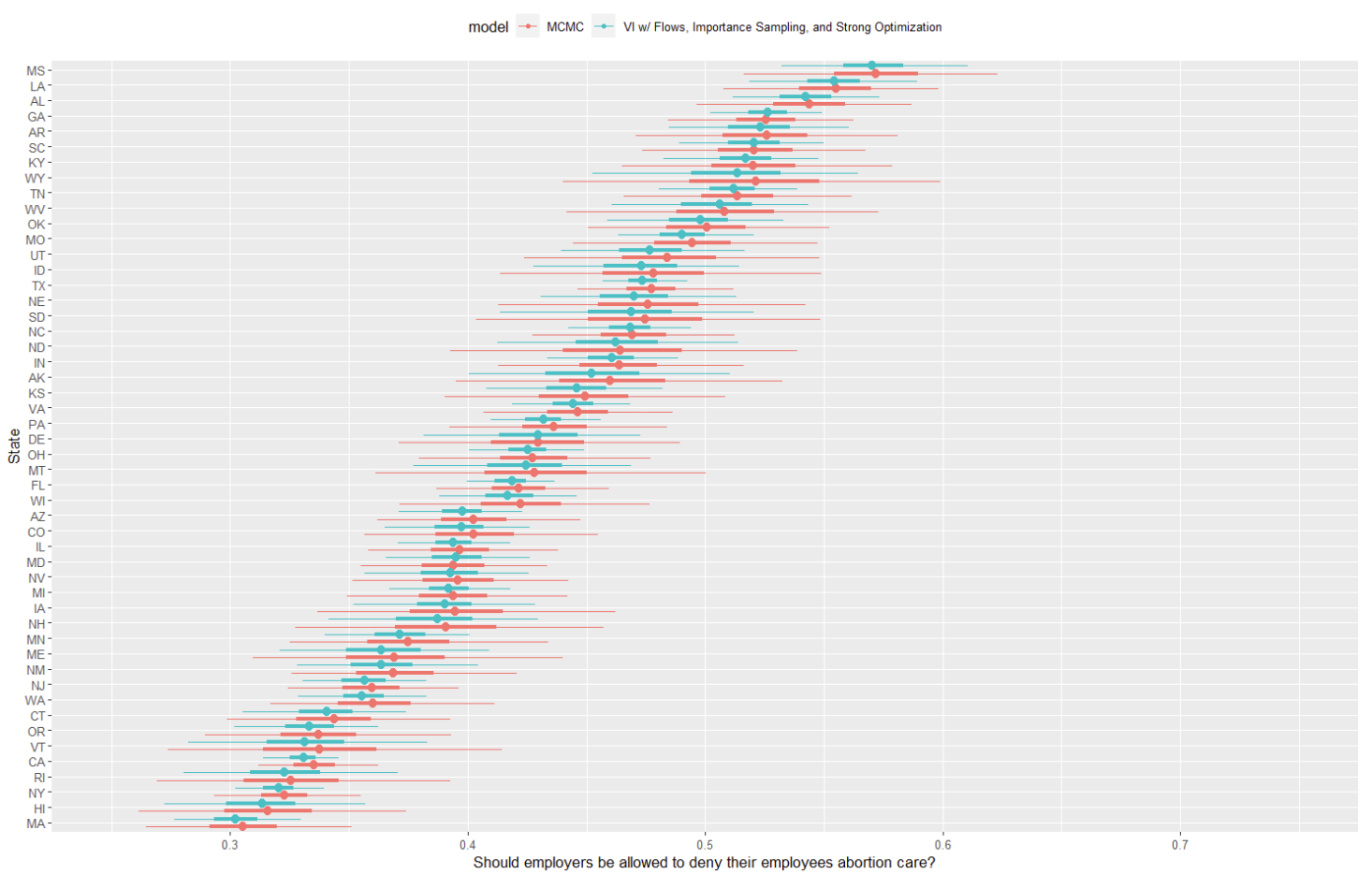
To cut to the chase, the new and improved variational approximation is looking pretty, pretty good!
Like with the simpler mean-field and full-rank models from earlier in the series, this has the medians basically correct, but we also have reasonable uncertainty estimation too. First, the state distributions are much more smooth and unimodal- no more “lumpy” distributions with odd spikes of probability that make no sense as a model of public opinion. Further, the approximation is more consistent: while there’s still some variation state to state in how closely VI matches MCMC, pretty much all states are reasonable.
Certainly, we’re still to some degree understating the full size of MCMC’s credible interval. Considering this model runs in an hour and change versus MCMC’s 8 hours on 60,000 datapoints (!), this feels pretty acceptable. As I’ll write a bit more about later, there are a few ways to trade compute and/or runtime to fill out the CI’s as well.
Last time we look at a variational approximation in post 2, we found a dot plot was a significantly more revealing visual, which made it clear how bad the first try at VI in the series was. How does that look here?
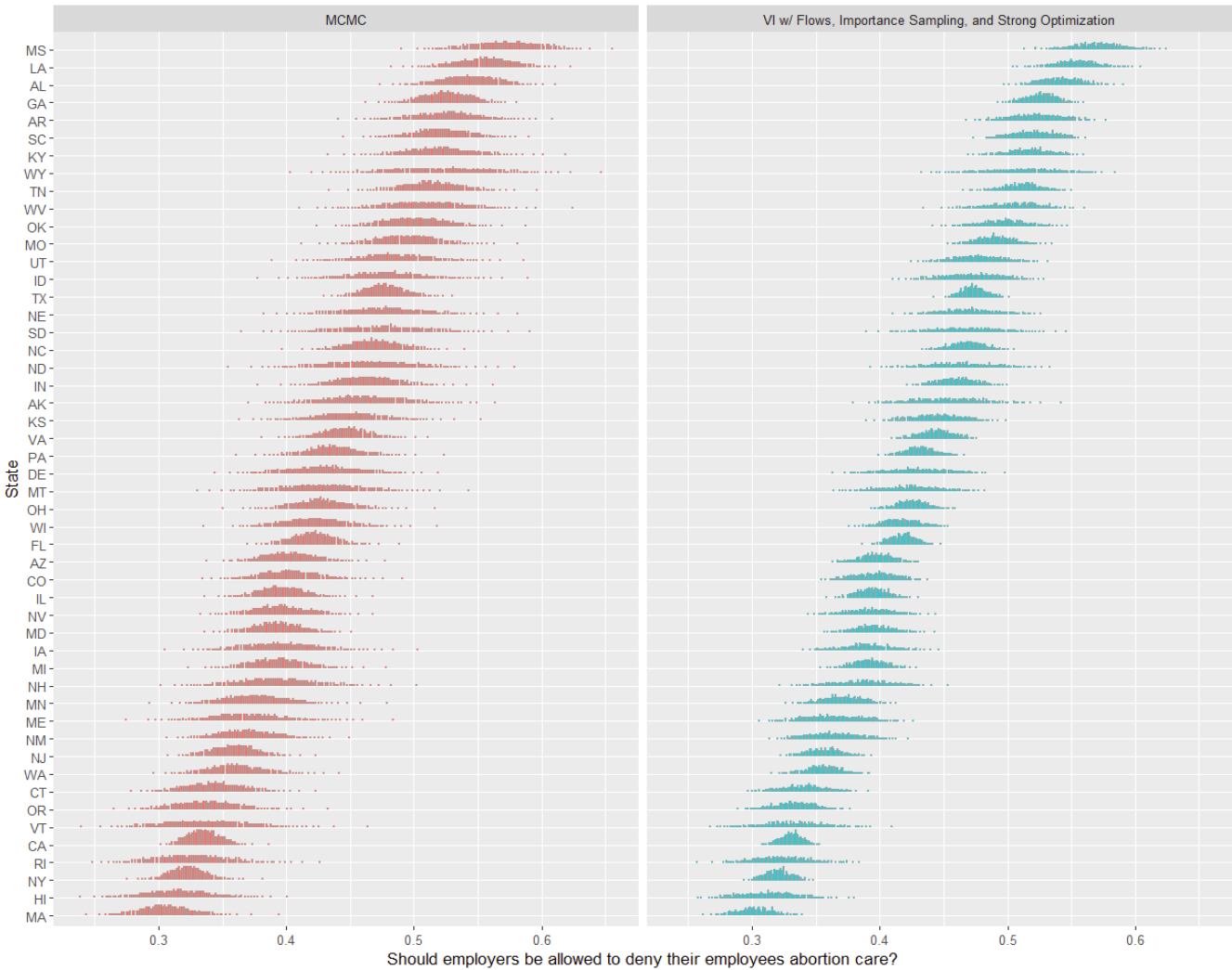
Again, pretty solid- no more weird spikes, and the concentration of mass looks pretty comparable (if a bit compressed) versus MCMC. VI is now much more uncertain about the same states as MCMC, and no longer shows any signs of degenerate optimization to fit data points. Nice!
Finally, how are the diagnostics we learned in the last post? The \hat{k} is .9, which is at least much improved1. The approximation is good enough that the Wasserstein bounds aren’t tight enough to inform us much about any issues2, although we should be a bit careful in trusting them giving that \hat{k} (recall: the Wasserstein bounds aren’t super reliable when \hat{k} is high). In one sense, none of the diagnostics here are “great”, but this is pretty typical of my experience with BBVI for non-trivial models. We’re almost always losing something from the true posterior, and these diagnostics are not sufficiently fine-grained to differentiate important from unimportant losses.
What worked here?
So the caption above gives some hints, but what all is in this model?
To fit this variational approximation, I’m using Agrawal, Domke, and Sheldon’s vistan, which is a companion python package to their great paper Advances In Black-Box VI.
Here’s a footnote with more implementation details3, but for purposes of this post, I’ll just reference the parameters of the main setup function here:
Let’s talk about:
- Normalizing Flows
- Importance Sampling
- Optimization
- Sampling Budgets
Normalizing Flows
First, this is using a Real NVP normalizing flow, with a fairly small (10) number of transformation layers, each of which is using a pretty shallow neural net (2 layers, 32 hidden units). This helps make the approximating distribution complex enough to handle our model. I didn’t find much benefit from either adding more transform layers or making the neural nets deeper- that sort of makes sense, since the jump from mean-field or full-rank VI to using a normalizing flow at all is a fairly big one in terms of model representation capacity.
Importance Sampling
Second, this is using importance sampling only at the sampling stage, and with just 10 IW samples per returned sample. I didn’t find much benefit from importance weighted training4 here, although for relatively more complex models than this I’ve found it to sometimes matter. As a point of comparison, in their paper linked above, Agrawal et al. find that about 20% of models actually get worse with IW-Training, and only ~10% get improvements, although those improvements seem to be clustered in more complex models and can be fairly significant.
At least for this particular model, using 10 importance samples per returned sample during provided most of the benefit of importance weighting, although pushing this higher to 100 or 200 helped fill out the outcome distribution’s tails a bit (more on this in a bit).
Optimization
Finally, many of the parameters here are about optimization, which we haven’t talked about in this series too much yet, despite it being critical to good performance.
First, Agrawal et al. found that variational inference is reasonably sensitive to optimization hyperparameters like the step size the Adam optimizer uses- to handle this, they suggest initial runs at few different step sizes (in step_size_exp_range), selecting the best one via an ELBO average over the whole optimization trace. This model benefits quite a lot from this, and Agrawal et al.’s results see strong improvements for ~25-30% of models using this adjustment.
Second, they use the Sticking the Landing (STL) gradient estimator, which I’ll link out to later, but is essentially removing the score term from the gradient to reduce it’s variance.
A final optimization hyperparameter here is the number of iterations (both for that step search procedure and the final run)- I found 1000 was more than sufficient for optimization of this model, with going up to 2000 iterations not getting us much benefit, but going down to 500 leading to a heavily over-dispersed posterior.
A sample budget?
Since their paper is ultimately a bakeoff, Agrawal et al.’s paper touches on the theme of a sample budget again and again, and it’s a great concept to consider here. Essentially, a sample or computation budget is somewhat fungible: given an amount of run time, compute available, etc, we can, for example, trade a larger max_iters for using (more) importance weighted training, or use fewer iterations for (more) importance weighting our samples.
How to best spend this budget is an open question and fairly model dependent- here, I decided not to present the best model I could possibly fit with variational inference, but the best one I could get to fit in ~1h. The point of this series is to fit something nearly as good fast, not a different, more complex way but also in 8h.
Next, I’ll talk through some ideas for what could improve the model further at greater compute and wall time cost.
What I might change next
The major shortfall of the current approximation (assuming we continue to mostly care about state level estimates) is the overly narrow credible intervals. If I did want to improve the accuracy of this model, what might I consider next?
The low hanging fruit here would be to use some combination of more samples and/or more importance weighted samples per retained sample. In my testing this produces credible intervals about halfway between what I showed above and the MCMC ones, at the cost of another hour of runtime. It might be possible to go further than this and get closer to the MCMC interval, but likely suffers from quite harsh diminishing returns. For some applications though, that might be the right trade off to make!
As I already mentioned above, I didn’t find much benefit from more training iterations, importance weighted training, or making the RNVP component deeper. Thus, if I wanted to really invest a lot of time to improve this further, my next step might be to consider fitting another model in parallel to ensemble with this one. For example, perhaps an objective like the CUBO that tends to emphasize coverage would be worth combining with this one either via multiple importance sampling or more simplistic model averaging.
What I might change for other models
A logical next question: for models in general, which situations suggest tweaking which hyperparameters? While this is a really hard question, I’ll offer some tentative thoughts:
The variational approximation is unable to represent the complexity of my model: In this situation, I’ve had the best luck increasing the complexity of my normalizing flow. Just like increasing the number of transforms helped in our ring density approximation example in post 6, more transforms and/or a deeper neural net within each transformation seems to be the most straightforward way I’ve found to improve representation capacity of variational inference. For the most complex models, perhaps changing the flow type will be necessary or efficient, but I’ve had surprisingly good luck just scaling up RNVP.
Like I mentioned above for this series’ specific model, I’ve had pretty meh results with IW-Training. I’ve had 1-2 models actually really benefit, but it hurts as often as it helps it seems, so it’s not something I reach for first anymore.
The approximation is close, but it misses some minor aspect the posterior: In this type of situation, like the one above, adding more samples or using more importance weighting to produce the samples has worked well. In my experience, diminishing returns on the number of importance samples kick in faster than on the number of full model samples. I rarely see benefits beyond a couple hundred importance samples, but more draws often continue to provide benefits well into the thousands sometimes. Keep in mind that having trained a VI model, sampling is often orders of magnitude faster than MCMC: “just sample more” is much less time consuming advice to take than with MCMC.
I can’t get the model to meaningfully converge: This often looks like the result we got in the second post in the series with mean-field and full-rank Variational Inference. Like with that post, there’s a variety of reasons this can happen. If you’re using mean-field or full-rank for a complex model, there’s a good chance you just need a normalizing flow or otherwise more complex approximating distribution to get any sort of useful convergence.
If you’re using something complex to make the approximation and you still see massively under/over-dispersed posteriors, then consider broadening the step size search, or grid searching a bit over the other Adam hyperparameters. Unlike with models based on deeper neural nets, I haven’t ever really seen a variational approximation plateau on loss for a long time and make a breakthrough; it’s pretty reasonable to trust early stopping and try to find something that actually gets optimization traction early on.
There’s a whole part of the posterior entirely missing: I’ve only really seen this with highly multi-modal posteriors, but sometimes a single ELBO based model will only meaningfully cover a single mode in a parameter you care about. In this case, I’ve found a few smaller models averaged/MIS’d together to be the simplest solution- a single model that covers all modes is often quite hard given the mode seeking behavior of the ELBO that I discussed in post 3. Trying a different loss here is an option, but for more complex posteriors, I often struggle to get convergence with the CUBO.
This is by no means a authoritative list, but hopefully this set of suggestions for the most common issues I’ve had with variational inference in a variety of applied models is helpful. I’d also highly recommend the Advances In Black-Box VI paper mentioned above for more practical guidance of this type.
Other things I didn’t cover
Variational Inference is a decent sized research area, so I couldn’t cover everything in this series. As a way to wrap up, I want to gesture at some other papers that are worthwhile, but weren’t worth a full post in this series.
Better Optimization for Variational Inference: Besides the work on step search in Advances In Black-Box VI, there are two really good papers on improving the underlying gradients we optimize on in variational inference. First, the Sticking the Landing gradient estimator removes the score term in the total gradient with respect to the variational parameters. The result is a still unbiased5, but lower variance gradient estimator which helps a lot with both normalizing flow and simpler approximation fitting. Second, for when using importance weighted training, there’s the doubly reparameterized gradient (DReG) estimator, which is both lower variance and unbiased via a clever (second) application of the reparameterization trick.
Pathfinder: Coming soon to brms and Stan in general, Pathfinder is an attempt at a variational inference algorithm by Lu Zhang, Andrew Gelman, Aki Vehtari, and Bob Carpenter6. It uses a quasi-Newtonian optimization algorithm, and then samples from (a MIS combination of) Gaussian approximations along the optimization. There’s a ton of clever work here to make this incredibly fast, and comparatively parallel versus other variational algorithms. For even moderately complex posteriors, it’s blazingly fast, and quite accurate.
My only problem with it is that for more challenging posteriors, I’ve found it a little limited: it doesn’t seem to have the representation capacity possible with normalizing flows, which unfortunately is necessary for most of the non-blog-post-series-examples applications I use VI for. Like so many papers with these authors though, there’s a ton here that’s deeply insightful and more broadly applicable knowledge here, even if you need normalizing flows for your work.
Boosting Variational Inference: Given how dominant boosting based algorithms are in basic machine learning, applying boosting to variational inference definitely had my attention when I first saw papers like Universal Boosting Variational Inference. What’s weird about this strain of papers though is that there don’t see to be any public replication materials that sufficiently implement this for me to test it out, and there are no comparative bake off versus other serious, modern variational inference algorithms I can find.
This may be a lack of familiarity on my part (and I’m most uncertain about boosting VI of everything I’ve discussed in this series), but the vibes of this sub-literature feel off to me. Why is no one releasing a public, serious implementation of this7? If the authors claims about performance and ease of use are true, this pattern of “lots of papers, little code” is even weirder. Again, I’m super uncertain here, but after investing some time to dig here, this corner of the variational inference literature is surprisingly hard to engage with, and so I haven’t really made the time yet.
Thanks for reading this end to the series! Writing it as I learned more and more about variational inference has been incredibly helpful to me, and hopefully it has been useful to you as well.
Footnotes
This is still not a “good” (< .7) \hat{k}, but as we saw in the last post, \hat{k} is not a infallible metric, especially if you are interested in just a summary or two of the posterior where any defects it suggests may not be relevant. My guess is that to get \hat{k} down, we’d need to move much further along in fully fleshing out the tails of the approximation, but even then we might still have issues given the dimensionality of this posterior.↩︎
This happens to me a lot, where these bounds don’t really tell me anything unless a model won’t even pass a basic smell test. If you have some counterexamples, I’d love to see them!↩︎
To fit this, I first used brms’s
make_standataon both the cleaned survey responses and the ~12,000 bin matrix we want to post-stratify on to get data to pass to Stan, which I just saved out as JSON files to read back in later. Then, I usedmake_stancodeto extract the basic Stan model, and added in logic to produce predictions onto the post-stratification matrix. You can see that modified Stan model here. After that, it was fairly easy to pass these inputs into vistan in python. One quick final note: vistan is quite sensetive to the version of python you use, so I recommend making a virtual environment with python 3.8 or 3.9.↩︎evaluation_fn = "IWELBO"is just a quirk of their syntax, where withM_iw_train = 1, it’s equivalent to not doing IW-weighted training at all.↩︎See the paper for a longer explanation for why it’s still unbiased, but essentially this term has expectation zero. for some samples it may not be zero, but it’s sufficient for the unbiasedness of the broader gradient that it have expectation zero.↩︎
See the paper for a longer explanation for why it’s still unbiased, but essentially this term has expectation zero. for some samples it may not be zero, but it’s sufficient for the unbiasedness of the broader gradient that it have expectation zero.↩︎
Beyond this toy example in Pyro, I can’t find much. Again, prove me wrong if you know of something.↩︎
Reuse
Citation
BibTeX citation:
@online{timm2023,
  author = {Timm, Andy},
  title = {Variational {Inference} for {MRP} with {Reliable} {Posterior}
    {Distributions}},
  date = {2023-07-12},
  url = {https://andytimm.github.io/posts/Variational MRP Pt7/variational_mrp_pt7.html},
  langid = {en}
}
For attribution, please cite this work as:
Timm, Andy. 2023. “Variational Inference for MRP with Reliable
Posterior Distributions.” July 12, 2023. https://andytimm.github.io/posts/Variational
MRP Pt7/variational_mrp_pt7.html.